|
1
|
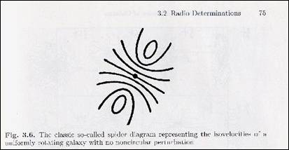
- Today: Kinematics and
Masses
- Unless noted, all figs and
equations from Combes et al. or Longair’s Galaxy Formation.
- WIRO…
|
|
2
|
- What are the relative advantages/disadvantages of each?
|
|
3
|
- What are the relative advantages/disadvantages of each?
- Radio has great velocity resolution.
- Radio sensitive to cool gas, beyond stars.
- Radio can map whole galaxy at once.
- Optical work used to be easier before VLA
- Optical work has, usually, better spatial resolution.
|
|
4
|
|
|
5
|
|
|
6
|
|
|
7
|
- Spirals -- no perfect solution with so much dark mass with somewhat
unknown distributions!
- Elliptical/spheroidal components treated, at least initially here, using
the virial theorem. Follow
Longair here, more detail.
Also no perfect solution.
- Order of magnitude, really.
Dark matter dominates.
|
|
8
|
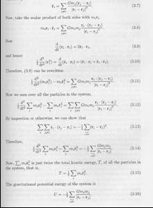
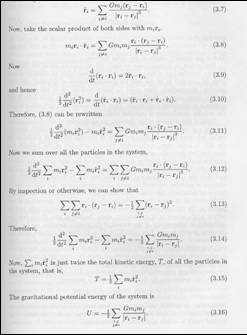
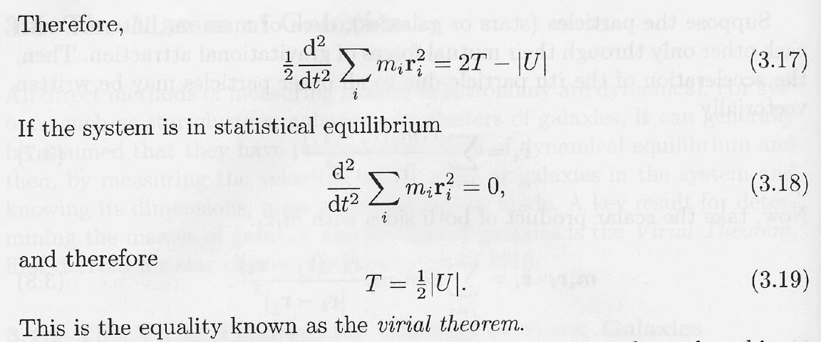
- Virial Theorem: A relationship between gravitational potential energy
and velocities for a dynamically relaxed and bound system.
- Ellipticals not necessarily rotating.
- T = ½ |U|, where T is the total kinetic energy and U is the
potential energy.
- So, for a cluster of stars or a cluster of galaxies, measuring T (by
measuring velocities) can give U and therefore M.
|
|
9
|
- Virial Theorem: T = ½ |U|
- You do need to worry about the conditions of the theorem in an
astrophysical context. For
instance, comparing crossing times with the relevant timescale. Text examples are the sun’s
orbital period and galaxies in Coma.
|
|
10
|
|
|
11
|
- Astronomical context more complex.
Cannot in general get all the 3D velocities. In exgal context, uncertain
cosmology can translate into uncertain spatial dimensions. Usually only have position on sky
plus radial velocities. Must
make assumptions about velocity distribution to apply virial theorem.
|
|
12
|
- Isotropic case: <v2> = 3<vr2> (why?)
- If velocity dispersion independent of masses:
- T = 3/2 M <vr2>, where M is total mass
- More complex if the above is not true. Assuming spherical symmetry and
an observed surface distribution, get a weighted mean separation Rcl:
|
|
13
|
- For the specific case of a sphere of total mass M, size R, and constant
density, the potential energy U = -3/5 (GM2/R). Thus the virial theorem says T =
½ U, so
- (3/2) M <vr2> = (3/5) GM2/R
- Mvirial = 5σr2R/G, where σr
is the radial velocity dispersion
- Works for elliptical galaxies and yields mass to light ratios of 10-20
in solar units.
|
|
14
|
- Textbook (Combes et al.) goes through the old approach of flattened
spheroids with a particular mass density as a function of radius. This is perhaps useful review for
qualifying exam as an exercise in gravitational physics.
- Key is to use the rotation curve.
- Solutions are appropriately simple for flat curves:
- M(total) = V2rot R/G (spherical dark matter)
- M(total) = (2/π) V2rot R/G (disk dark
matter)
- Where the disk is cut off at r=R, and V = constant (flat curve) inside
r < R.
- Mass increases linearly with r, for V = constant
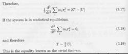
- Mass/Light ratio increases faster
|
|
15
|
|
|
16
|
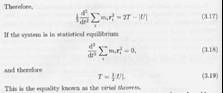
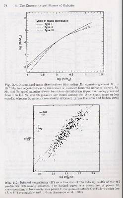
- The famous Tully-Fisher law (basically L ~ V4). Mike Pierce is an expert. Why is H-band better and why is
this so important in extragalactic astronomy?
- What is its origin?
|
|
17
|
- M(total) = V2rot R/G
- Recall M/L = constant (at least within class – and is more true
across classes for H-band)
- L ~ V2rot R/G
- Also, surface brightness, μ, L/R2 ~ constant
(“Freeman’s Law,” μ(r) = μ0exp(-r/r0))
- Spiral central surface density = 21.65 B-mag arcsec-2
- Together these give L ~ V4, or in terms of Absolute
magnitude, M = -10logV + constant
- Next chapter, Faber-Jackson equivalent for ellipticals
|
|
18
|
- Large Scale Distribution of Clusters
- Galaxy Distribution in Clusters
- Dark Matter in Clusters
- Forms of Dark Matter
- (Combes et al. covers this way too briefly in ch. 11, so something of an
aside now.)
|
|
19
|
- Palomar Sky Survey using 48 inch Schmidt telescope (1950s)
- Abell (1958) cataloged “rich” clusters – a famous work
and worth a look
- Abell, Corwin, & Olowin (1989) did the same for the south using
similar plates
- All original work was by visual inspection
|
|
20
|
|
|
21
|
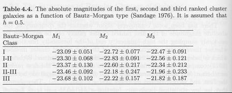
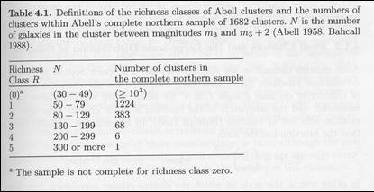
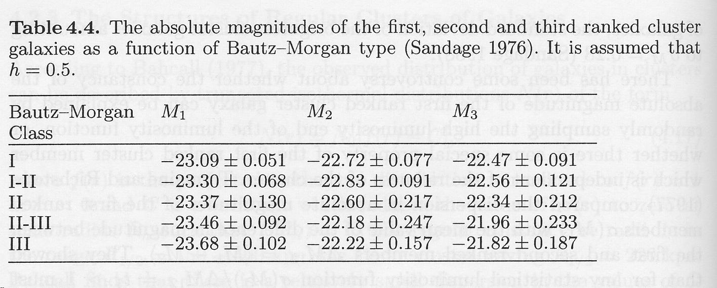
- Richness Criterion: 50 members brighter than 2 magnitudes fainter than
the third brightest member. Richness
classes are defined by the number in this range:
|
|
22
|
- Compactness Criterion: Only
galaxies within an angular radius of 1.7/z arcmin get counted. That corresponds to a physical
radius of 1.5 h-1 Mpc.
The redshifts are (were) estimated based on the apparent
magnitude of the 10th brightest cluster member.
|
|
23
|
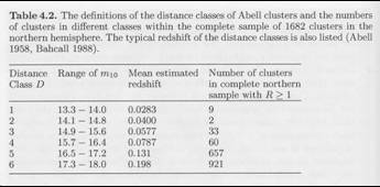
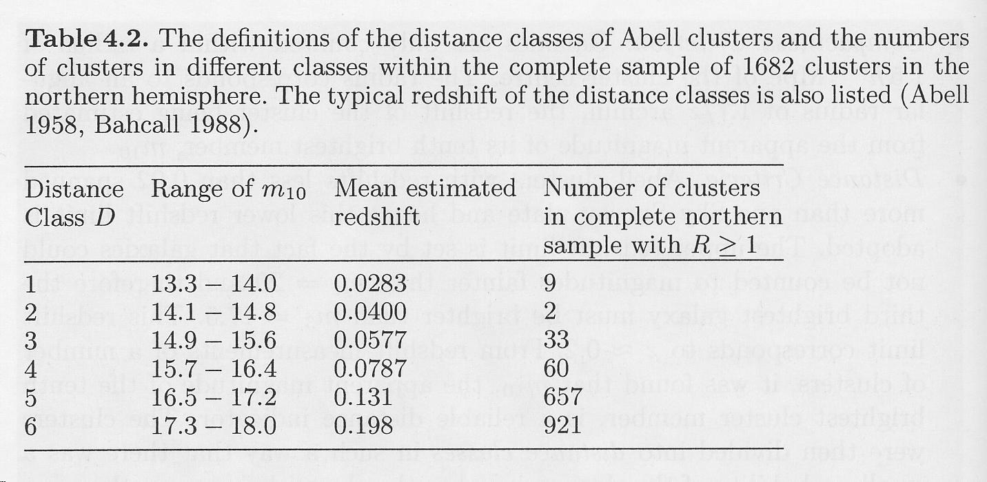
- Distance Criteria: Lower
redshift limit (z = 0.02) to force clusters onto 1 plate. Upper limit due to mag limit of
POSS, which matches z of about 0.2.
Distance classes based on magnitude of 10th member:
|
|
24
|
- Complete Northern Sample:
- 1682 Clusters of richness 1-5, distance 1-6.
- Counts in Table 4.2 follow:
- This is consistent with a uniform distribution*.
- Space Density of Abell Clusters richer than 1:
- For uniform distribution, cluster centers would be 50 h-1
Mpc apart, a factor of ten larger than that of mean galaxies.
|
|
25
|
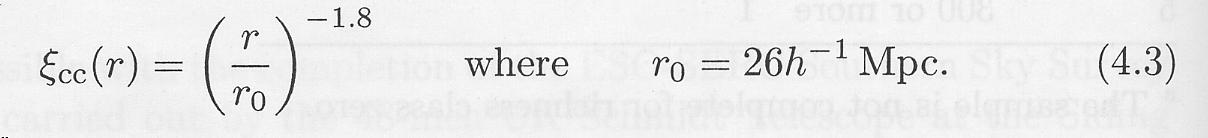
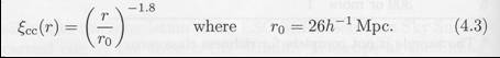
- Based on Abell’s Northern Sample:
- Spatial 2-point correlation function (Bahcall):
- Scale at which cluster-cluster correlation function has a value of
unity is 5 times greater than that for the galaxy-galaxy correlation
function.
|
|
26
|
- Peebles (1980) schematic picture:
- Cloud of galaxies is basic unit, scale of 50 h-1 Mpc
- About 25% of galaxies in these clouds
- All Abell Clusters are members of clouds (with about 2 per cloud), and
contain about 25% of the galaxies in a cloud are in Abell Clusters
(superclusters occur when several AC combine)
- Remaining 75% follow galaxy-galaxy function
- In terms of larger structures, galaxies hug the walls of the voids,
clusters at the intersections of the cell walls.
|
|
27
|
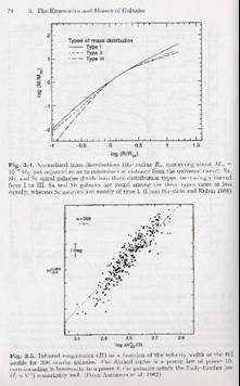
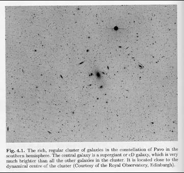
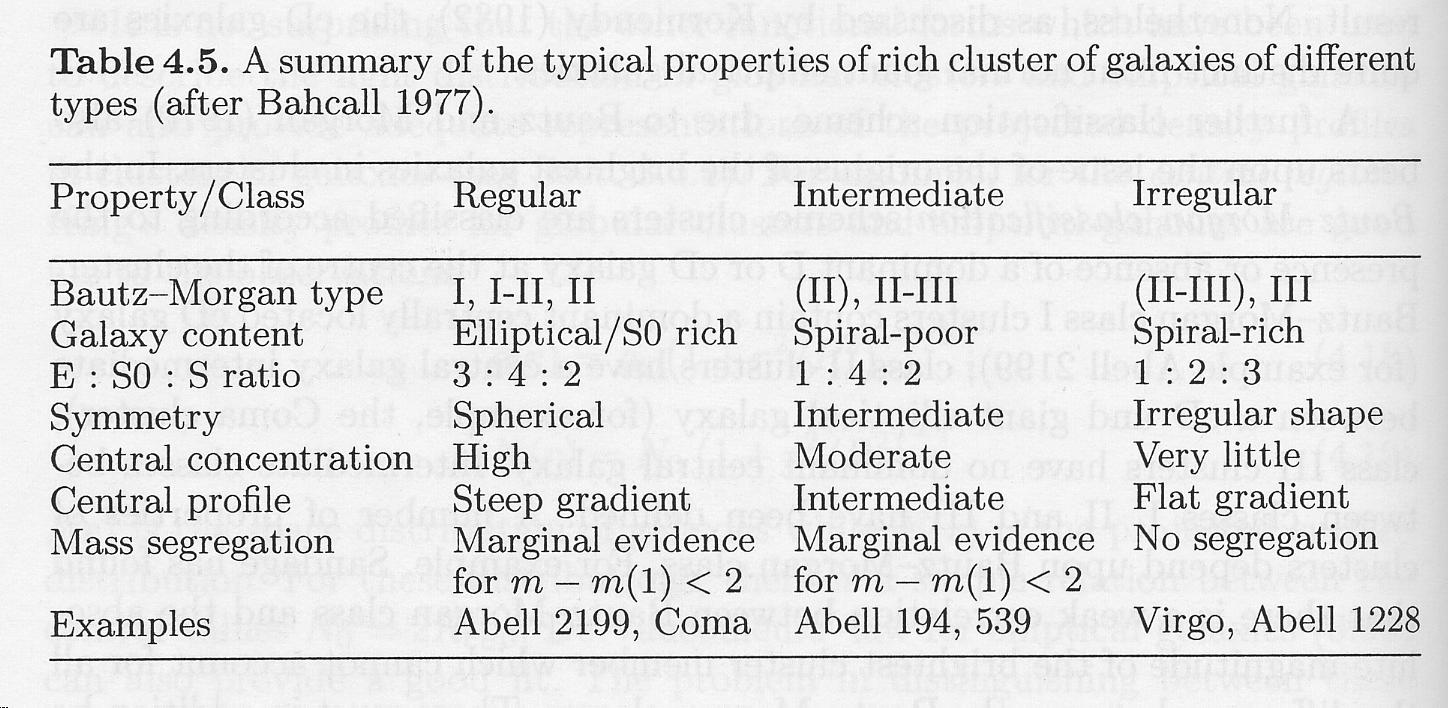
- A range of structural types (Abell)
- Regular indicates cluster is circular, centrally concentrated (cf.
Globular clusters), and has mostly elliptical and S0 galaxies. Can be very rich with > 1000
galaxies. Coma is regular.
- All others are irregular (e.g., Virgo).
- I don’t know why he didn’t just call them type 1 and type
2…! /sarcasm
|
|
28
|
- A range of structural types (Oemler 1974)
- cD clusters have 1 or 2 central dominant cD galaxies, and no more than
about 20% spirals, with a E: S0: S ratio of 3: 4: 2.
- Spiral-rich clusters have E : S0 : S ratios more like 1: 2: 3 –
about half spirals.
- Remainder are spiral-poor clusters. No dominant cD galaxy and
typical ratio of 1: 2: 1.
|
|
29
|
- Galaxies differ in these types (Abell)
- In cD clusters galaxy distribution is very similar to star distribution
in globular clusters.
- Spiral-rich clusters and irregular clusters tend not to be symmetric or
concentrated.
- Spiral-poor clusters are intermediate cf. above.
- In spiral rich clusters, all galaxy types similarly distributed and no
mass segregation, but in cD and spiral-poor clusters, you don’t
see spirals in the central regions where the most massive galaxies
reside.
|
|
30
|
- Bahcall (1977) describes distributions as truncated isothermal
distributions:
- Where f(r) is the projected distribution normalized to 1 at r=0, and C
is a constant that makes N(r) = 0 at some radius. Results in steepening
distribution in outer regions vs. pure isothermal soultion.
- R1/2 = 150-400 kpc (220 kpc for Coma)
|
|
31
|
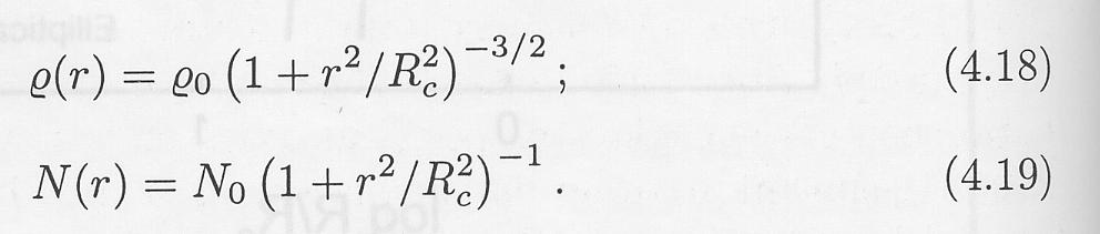
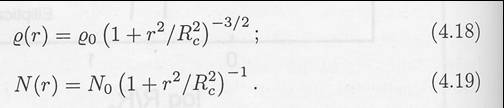
- In central regions King profiles work well:
- For these distributions N0 = 2Rcρ0.
- De Vaucouleur’s law can also work.
- Problem is observations do not constrain things quite tightly enough.
|
|
32
|
|
|
33
|
|
|
34
|
- How do we know it is there?
- Dynamical estimates of cluster masses
- X-ray emission/masses
- (Sunyaev-Zeldovich Effect)
- (Gravitational lensing)
- What is the dark matter???
|
|
35
|
- Dynamical estimates of cluster masses
- Virial Theorem as we have discussed, but…
- Very few clusters exist that can be well done!
- E.g, which are cluster members?
- Must measure many velocities
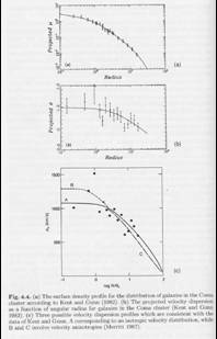
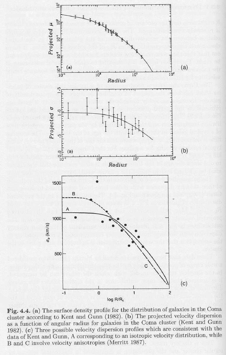
- Case of Coma
- Regular rich cluster, looks like isothermal sphere
- Crossing time arguments OK
- Virial mass issue for Coma first by Zwicky (1937)
- Surface distribution, velocities in next figure…
|
|
36
|
|
|
37
|
- Merritt (1987) analysis:
- Assuming constant M/L ratio, then mass is 1.79 x 10¹⁵h-1
solar masses, and M/L is 350 h-1 in solar units (think about
that!).
- Typical M/L for ellipticals is 15 in solar units.
- Differ by a factor of 20
- Why should the dark matter have the same distribution as the light?
- Why should the velocities even be isotropic?
|
|
38
|
- UHURU in 1970s:
- Rich clusters very bright in X-rays!
- Bremsstrahlung emission of hot intercluster gas
- Very hot gas requires large potential to hold
- Can use to estimate the cluster mass
|
|
39
|
- Fabricant, Lecar, and Gorenstein (1980, ApJ 241, 552):
- Assume spherical symmetry (as usual!)
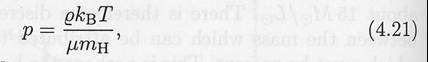
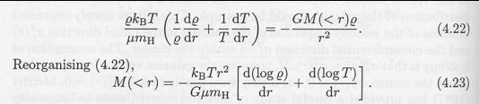
- Assume hydrostatic equilibrium (yes!):
- Perfect gas law:
|
|
40
|
- Fabricant, Lecar, and Gorenstein:
- For ionized gas, cosmic abundances, μ = 0.6
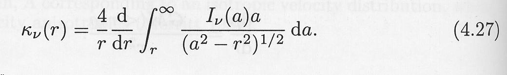
- Differentiating the gas law, and inserting into the hydrostatic
equation:
- So, the mass distribution can be found if the variation of pressure and
temperature with radius are known (measured).
|
|
41
|
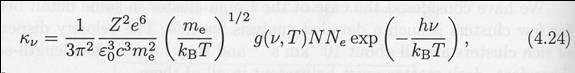
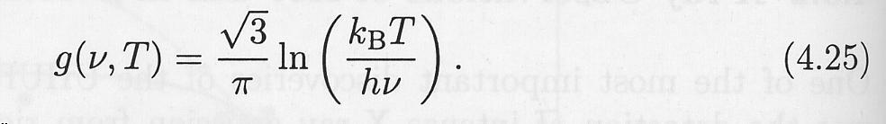
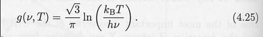
- Fabricant, Lecar, and Gorenstein:
- Bremsstrahlung spectral emissivity:
- Gaunt factor can be approximated:
|
|
42
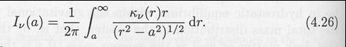
|
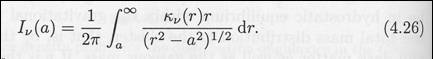
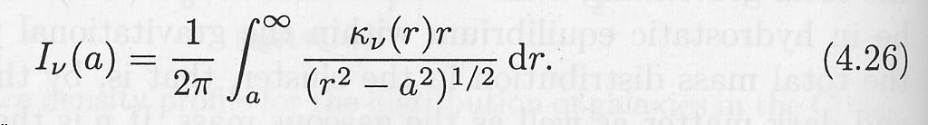
- Fabricant, Lecar, and Gorenstein:
- Bremsstrahlung spectrum is roughly flat up to X-ray energies, above
which it cuts off exponentially.
Cut-off is related to temperature. E = hν ~ kBT. The measurement is a projection
onto 2D space. Integrating
emissivity and converting to intensity (surface brightness at the
projected radius a):
|
|
43
|
- Simplified procedure:
- Luminosity Density = total energy per second per unit volume
integrating over all frequencies, for a fully ionized hydrogen plasma:
- Lvol = 1.42 x 10⁻²⁷ne2T1/2
ergs/s/cm3
- Sometimes it can be assumed that you have an isothermal sphere (which
is the case when the dark matter and the gas have the same radial
dependence). More next week
on this.
|
|
44
|
- So, from the spectrum we can get the temperature as a function of
radius, and from the intensity we can get the emissivity and hence the
particle density.
- Chandra is great for this type of observation:
- http://chandra.harvard.edu/photo/2002/0146/
- http://chandra.harvard.edu/photo/0087/
- http://www1.msfc.nasa.gov/NEWSROOM/news/photos/2002/photos02-037.html
- Cooling flows are one possible complication.
|
|
45
|
- ROSAT pictures: old and busted.
- Chandra images: The New Hotness.
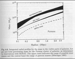
- Important result is that the dark matter does follow the galaxies.
- Typical masses then are 5x10¹⁴-15 solar masses, only 5%
visible light, 10-30% hot gas, rest is DM.
|
|
46
|
- We’re certain it is present.
- Some is baryonic.
- More is non-baryonic.
|
|
47
|
- Protons, Neutrons, electrons (include black holes here too).
- “Bricks?”
- Brown dwarfs and the like.
- BB nucleosynthesis constrains baryons to less than 0.036 h-2
of closure density.
|
|
48
|
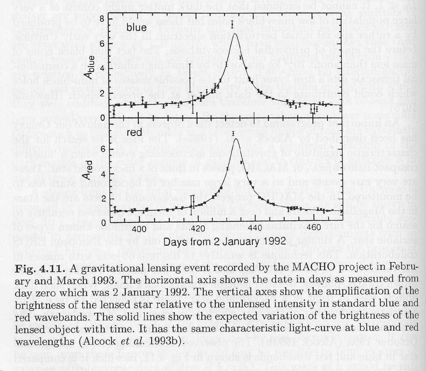
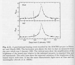
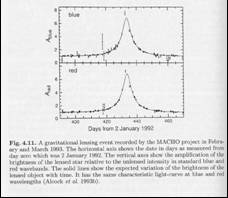
- Black holes constrained by lensing effects (or lack thereof).
- MACHOs (Alcock et al. 1993):
|
|
49
|
- MACHOs:
- http://www.owlnet.rice.edu/~spac250/coco/spac.html
- MACHOs are rather massive, around half a solar mass, and can contribute
up to half of the dark halo mass.
- White dwarfs???
|
|
50
|
- I’m no expert on this stuff (and in some sense NO ONE is). Particle physicists play in this
area more than astronomers.
- Leading candidates include
- Axions. Cold, low mass,
avoid strong CP violation.
- Neutrinos. Hot, low mass
(getting better constrained), lots of them. SN helps.
- WIMPs. Gravitino, photino,
etc.
- Mirror Matter.
|

 Notes
Notes